Office Hours #1: Simulating from mixed-effects models

Not all requests can be videos, but I can still respond to them

Sometimes, I get comments on my YouTube videos asking about more advanced topics. Until now, I didn’t know how to help these people because I have my own internal schedule for my videos. So, I’m going to dedicate a new series to helping these commenters out. I'll be calling this series “Office Hours”.

A while back, someone asked me about simulating for mixed-effects models! Here’s the comment below for reference, probably hard to read.

While I’ve never done a sample size calculation directly for a mixed-effects model, I thought it would be cool to try it out here.

The Model

Mixed-effects models are one of the most widely used statistical tools. They’re useful for accounting for clustering in data and can even be used for longitudinal analysis.

Below is a mixed-effects model for a continuous outcome. Note that there can be mixed-effects models for binary or count outcomes (i.e. GLMMs).

\(Y_i = (\beta_0 + b_{i0}) + X_i (\beta_1 + b_{i1}) + \epsilon_i, \quad \begin{pmatrix} b_{i0} \\ b_{i1} \end{pmatrix} \sim N_2(0, G), \epsilon_i \sim N(0, \sigma^2_{\epsilon})\)

This model has a similar form to a standard linear regression, but has a crucial new addition: subject-specific terms. These are indicated by the lower-case “b” terms, and you can see they have subject-specific indices indicated by the “i”.

These new terms indicate the each individual can “vary” somewhat from the population-level regression terms (the beta parameters). The population-level terms are also confusingly known as the “fixed” effects, and the subject-specific parameters are known as “random” effects. These “fixed” and “random” effects give the mixed-effects models their name. Most often, we are interested in learning more about the fixed effects, because they represent our population-level parameter.

The subject-specific effects are assumed to come from a Normal distribution. Given a person’s specific effect, the distribution of their outcomes are:

\(Y\mid \mathbf{b}_i \sim N(\beta_0 + b_{i0} + X(\beta_1 + b_{i1}), \sigma^2_{\epsilon} )\)

Allowing observations to have their own specific effect makes for a very flexible model.

So how do we simulate from one?

Code: Random intercept

Here’s the code for a simpler version of the mixed-effects model, the random intercept model. Here, only the intercepts have subject-specific deviations:

\(Y_i = (\beta_0 + b_{i0}) + X_i \beta_1 + \epsilon_i, \quad b_{i0} \sim N(0, \sigma^2_b), \epsilon_i \sim N(0, \sigma^2_{\epsilon})\)

J = 10                # number of individuals
n_j = 30              # number of observations per individual 
sigma_b = 5           # variance of the random intercept
sigma_e = 1           # variance of the random noise
fixed_effect = 1      # population-level effect
fixed_intercept = 5   # population-level intercept

data = tibble(
  subject_id = 1:J,
  
  # Generate subject-specific intercept deviations
  b_i = rnorm(J, mean = 0, sd = sigma_b),
  
  # Generate uniform predictor (easier to visualize)
  X = map(subject_id, function(id) {
    runif(n_j, min = 0, max = 10)
  }), 
  
  # Generate outcome from predictor & subject-specific intercept
  Y = map2(b_i, X, function(bi0, x) {
    (fixed_intercept + bi0) + fixed_effect  * x + rnorm(n_j, mean = 0, sd = sigma_e)
  }) 
) |> 
  unnest(c(X, Y))

At the top, I’ve listed all the different parameters that we can control for a simulation study. First, I generated the random intercepts and then used these when generating the outcomes for each individual.

A plot of the data should look similar to the following:

Visualization of the simulated data from a random-intercept model

Notice that each of the lines are approximately parallel (due to the common slope), but they differ on the intercept. This is characteristic of the random-intercept model.

Code: Random intercept and slope

Here’s another bit of code for the more general model I showed earlier. It’s also referred to as a “random intercept and slope” model because both the intercepts and slopes are allowed to have subject-specific deviations.

J = 10                                  # number of individuals
n_j = 30                                # number of observations per individual 
G = matrix(c(10, 0, 
             0, 10), nrow = 2)          # covariance matrix of random-effects
fixed_effect = 1                        # population-level effect
fixed_intercept = 5                     # population-level intercept

# Generate random effects first from multivariate normal
random_effects = mvrnorm(J, mu = c(0, 0), Sigma = G) |> as_tibble()
names(random_effects) = c("b_i0", "b_i1")

data = random_effects |> 
  mutate(
    subject_id = 1:J,
    X = map(subject_id, function(id) {
      runif(n_j, min = 0, max = 10)
    }), 
    
    # Generate outcome from predictor & subject-specific intercept and slope
    Y = pmap(list(b_i0, b_i1, X), function(bi0, bi1, x) {
      (fixed_intercept + bi0) + 
        (fixed_effect + bi1)  *  
        x + rnorm(n_j, mean = 0, sd = sigma_e)
    }) 
  ) |> 
  unnest(c(X, Y))

And here’s a similar visualization of the resulting data:

Visualization of data from a random intercept and slope model

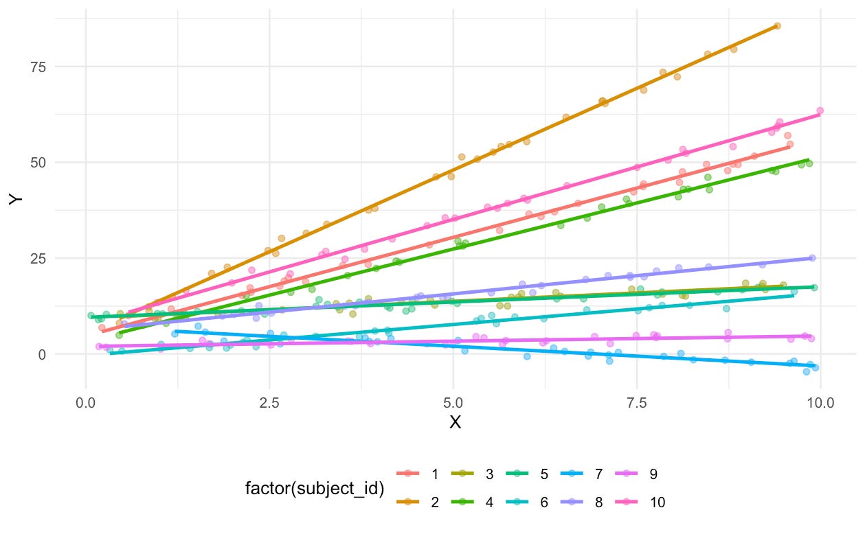
To generate the random effects, we need to sample from a multivariate normal instead (via mvrnorm from the MASS library). Afterwards, we generate the outcomes based on the linear model and each subject’s specific effects. It’s harder to see that the intercepts vary, but we can clearly see that each person has a different slope.

If you’d like a copy of the code for both the simulation and the visual, you can find it in this Github repo.

Things to investigate

After the data is generated, you can use a standard mixed-effects library like lme4 or nlme to estimate the model from the data. From there, you can record results from the hypothesis tests on the population-level parameter for checking type-I error, power, and sample size calculations.

In a mixed-effects model, there are quite a few knobs you can turn:

• The number of subjects/clusters in the study

• The number of observations per subject

• The values for the fixed effects

• And the variance structure of the random effects

A sample size calculation would focus on the fixed effects, but you’d most likely be interested in a sample size for an effect size (ratio of fixed effect to noise).

Hope this was helpful! This was a nice change of pace to my weekly rambles on the YouTube channel and my workflows. See you next week.

Christian

---

Current State of The Channel

😵‍💫 What am I working on right now?

• I’m currently editing an explainer video for part 1 of a 2-part series on basic nonparametric tests

🧐 What am I enjoying right now?

• Book — I thought it would be a good idea to listen to books about teaching since, to be honest, I am going off of instinct when I write my scripts. I want more principled approaches, especially since I want to develop my own courses. What I’m currently listening to is Uncommon Sense Teaching: Practical Insights in Brain Science to Help Students Learn by Barbara Oakley and Beth Rogowsky.

• Thing — I got a camera! You’ll be seeing my face a lot more, and less stock footage (as soon as I figure out a good green screen set up).

📺 What are my recent videos?

• 5 tips for getting better at statistics: a video detailing some of my best practices for learning statistics, honed from struggling in graduate school

📦 My other stuff

• I wrote guided solutions to problems to Andrew Gelman’s Bayesian Data Analysis. It’s for advanced self-learners teaching themselves Bayesian statistics

Heads up! Some of the links here are affiliate links, so I may get a small amount of money if you buy something from them. I only link stuff I actually use.