Probability Distributions Explained
Developing a mental map for probability distributions

This blog post is a lightly edited version of a video I posted on Youtube. If you’d like to watch instead, go for it! Otherwise, feel free to continue reading.
Introduction
In this post, we’ll talk about probability distributions. We'll talk about what they are, why they're important, and we'll use a little bit of code along the way.
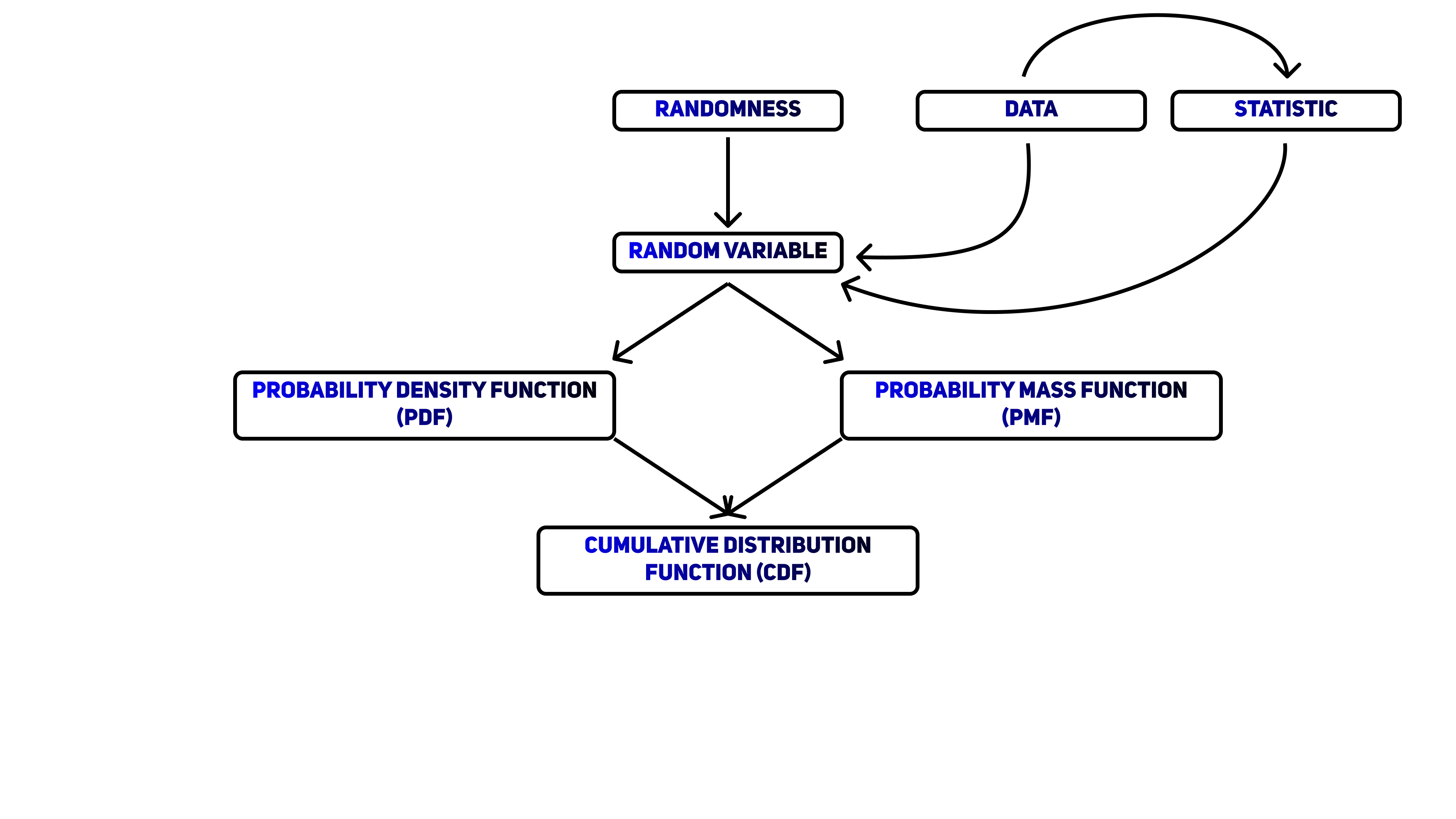
These are the main concepts and ideas we will use throughout this video. At the end, we'll weave each of them into a simple mental map.
Randomness
Random variable
Probability distribution
Probability mass function
Probability density function
Cumulative distribution
Data
Statistic
The world is a random place. Sometimes you win, sometimes you lose. Sometimes, your Uber driver talks to you, and other times they’ll talk to you even when you paid a little extra for them to not say anything. We'll define randomness as the presence of uncertainty, or even better, the absence of predictability. Randomness means that no matter how hard you try, you can't perfectly predict what will happen next.
This unpredictability kind of sucks. Our brains are trained to search for patterns, and it doesn’t take much to convince us that something is happening when it actually isn’t. Think of lucky steaks in the casino or the supposed hot-hand in basketball. Our pattern finding brain sees these trends and believes that some force is causing these things to happen when, like our own luck or Stephen Curry's skill. In reality, both of these things are just a string of random events that we interpret to be non-random.
This brings up a problem. If we can see patterns in the world that aren't actually there, how do we distinguish these illusions from actual trends that exist? To understand this, statisticians use mathematical models to try to impose structure on this randomness. To understand what we mean by "structure", we need to understand the probability distribution, which is the main focus of this training video. But before we get to that, we need to learn about the random variable.
Random variables
One of the basic elements of a statistical model is the random variable. If you were to read about random variables in a textbook, you would see that a random variable is a function. This function takes elements in a sample space of an event and outputs a number. That’s it. There are more formal definitions of a random variable, but those definitions aren't that helpful to us as statisticians.
Instead, we'll ground our understanding in a few examples.
As a first example, let’s say that we're playing a game of Catan, a board game that's been the source of a lot of bitterness in my life. You don't need to know the rules of Catan, only that the main source of randomness in the game is the roll of two six sided dice. After you roll, you take the sum of the two dice. The outcome of this sum decides whether or not you get resources, which lets you do stuff in game.
This matrix shows the possible sums from two dice:
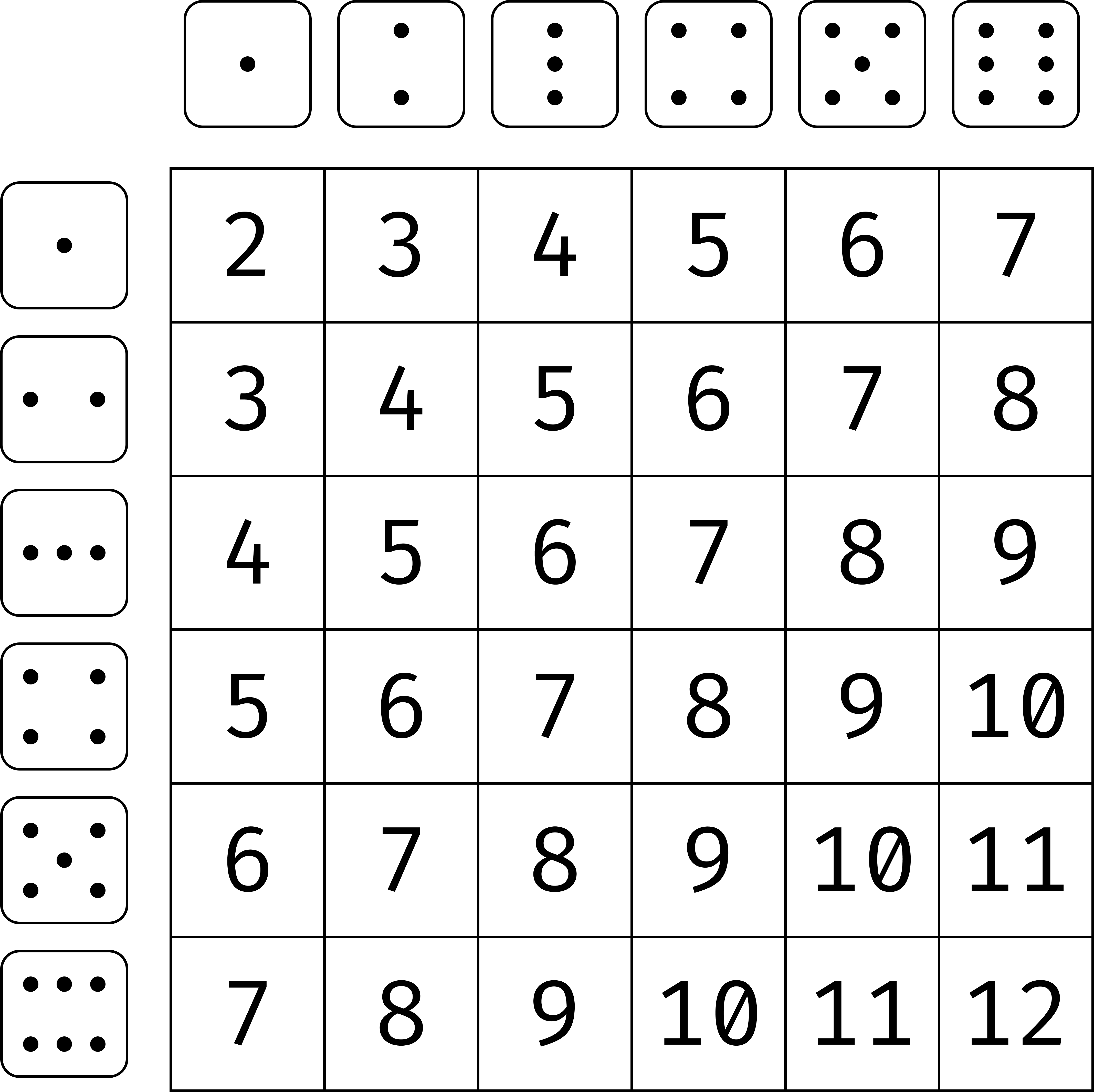
We can see that their sum can range from 2 to 12. Due to randomness, we can't know which one we'll get ahead of time. Some of you may already see which sums are more likely and which ones aren't. We'll get to that.
For our second example, let's say the thing I want to observe is the hours of watch time that this Youtube channel gets in a day. Hours is a measure of time, so the range of possible values is, theoretically, infinite. But only infinite in the positive direction.
As a final example, let's say the thing I want to observe is whether or not you finish my Youtube video. Since I know you will, the only value this random variable can take is 1, the number I use to represent the idea of “yes”. But, theoretically, some of you won’t finish the video, sp this random variable can also be 0, used to represent the idea that an event didn't happen.
The central takeaway is that random variable is a mathematical representation of something in the world that can take a range of numerical values, but we can’t predict what value we’ll see in advance.
These values can be discrete, as we saw in the first and third example, or continuous, as we saw in the second example.
You'll need to be familiar with a bit of notation. When a random variable is a capital letter, we are conveying this object can take on different values.
When we see a lower-case version of that same letter, we have actually observed a value from the random variable.
It's no longer random since it's something we have observed.
Probability Distributions
We now know that a random variable can take on different values, but just knowing the range of values isn't that useful. We might also be interested in knowing how likely we are to see these different values.
For example, in Catan, there is a map of hexagons, and most of these hexagons have numbers on them. If you have property on a hexagon, you can collect resources, but only if the sum of the dice roll matches that number.
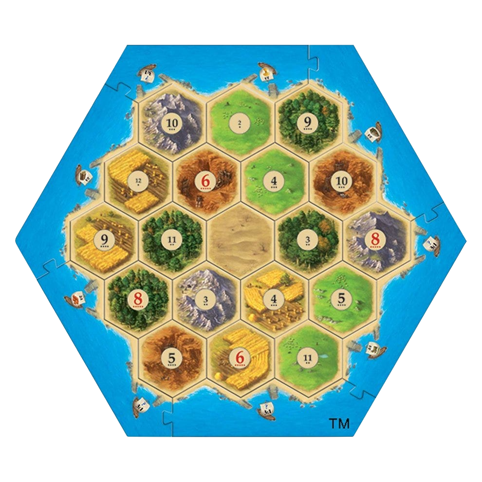
Therefore, it's in your best interest to choose numbers that are more likely to come up. Otherwise, you're just sitting there eating Doritos while everyone else is gathering sheep.
To be more precise, what we want is a function. This function will take in a number, and it will output another number. This output number will describe to us how likely we are to see the input number. If this output is higher, it means that that we're more likely to observe that input number. If the output is zero, then we can interpret this as it being impossible to observe that input.
Luckily, all random variables have such a function, which we refer to as the probability distribution. It may also be called the probability density function - or PDF - or the probability mass function, or PMF, depending on if the values we observe are continuous or discrete. From here on, I'll use the phrase "probability distribution" and I'll denote this function with a lower-case f.
The probability distribution is important because it's what describes the structure in the randomness in a random variable. To understand what I mean by this, let's look at the probability distribution of the double dice roll sum. The distribution takes on this triangle shape:
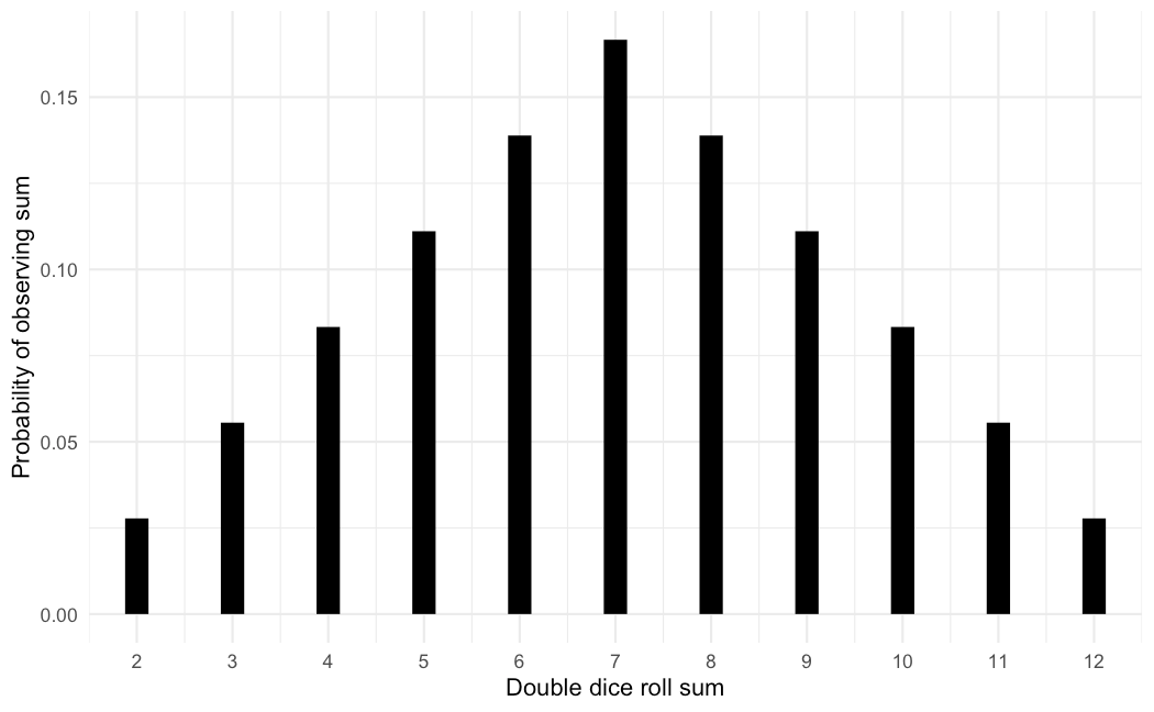
When many people think of randomness, they often think of chaotic, unpredictable static. If we know the probability distribution, then we'll know that this randomness at least has predictable structure.
The heights of the function tells us how likely each value is. By looking at the entire function, you can see which values are likely and which are not. If you want more resources, choose hexagons with 8 or 9. If you want to have a bad time, choose 2 or 12. We can even evaluate the probability distribution for sums that are impossible to observe, like 1 or 13. To convey that these sums are impossible, the height of these sums are zero. Only the possible sums have values associated with them.
Some of you may have noticed this, but I've avoided using the word "probability" to describe the output of the probability distribution. That word does apply in the case of the PMF, but not in the PDF. With a PMF, you can get a probability from both point values and a range of values. To get the probability of a range of values in a PMF, you just need to add the outputs of these values. If you want to get a probability from a PDF, you have to talk about a range of values. If you take a point value from a PDF, it's not a *probability*. It's technically a probability density. It can still tell us that one value is more or less likely than another, but it's not a probability.
But no matter what you have, PMF or PDF, the important takeaway is that the height of the probability distribution tells you about how likely that value is. The same logic will apply to ranges of values. The probability of observing any of the possible values should be 100%, and like its name suggests, the probability distribution tells us how probability is divvied up across these values. That's what I mean by structure.
Cumulative distribution
It's worth mentioning there is an alternative way to describe the structure of randomness in random variables. It's a close cousin to the probability distribution, and its called the cumulative distribution function. Note that the "d" in PDF and the "d" in CDF are not the same word. This will come up again when we look at some code.
Like the PDF and PMF, the CDF takes in a number and outputs a particular kind of probability. The CDF gets its name from the fact that it outputs a cumulative probability, the probability that a random variable will be less than or equal to a given value. We usually denote the CDF with an upper-case F.
Many people prefer to work with the probability distribution, but the CDF enjoys the benefit of always outputting a probability so I don't need to be so careful with my phrasing. In fact, the CDF conveys the same information as the PDF, but it just takes some effort to see. I'll demonstrate here with the double dice roll example since this relationship is easier to see with discrete random variables.
The CDF of the double dice roll looks like this:
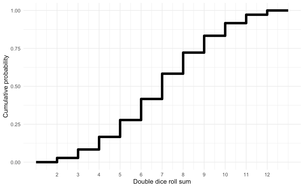
CDFs of discrete random variables always take on this staircase appearance. For reference, I'll also have the PMF to the side. Before the number 2, the CDF outputs a value of zero. But once we reach 2, we jump to 1/36. When we get to 3, we jump to 3/36. At this point, we need to add the probabilities of the sum being 2 and the sum being 3, since the CDF outputs the cumulative probability. Therefore, these jumps indicate how much probability is allocated to that number. A bigger jump means more probability which means that value is more likely. So these jumps help to describe the structure of the randomness, as the height does in the probability distribution.
Probability and statistics
Before we look at some code, let’s talk about a connection between probability and statistics. They're very often paired together, but the distinction between them is not made clear. When people first start learning about probability distributions, they are grounded in real world examples like the dice I mentioned. These are good for first picking up the concept of random variables, but I feel they don't help explain why we statisticians would bother to learn about it.
Let me ask. What are the random variables we deal with in statistics?
The first is the dataset. Data is a really general, but I'll use it to represent observed information in number form. When we collect data, it usually comes in the form of a sample. A dataset is just a collection of observed random variables. The number of observations, or sample size, is usually denoted with the letter n. A dataset is observed, so we usually denote it like this. If we're just talking about the general idea of a dataset, then it would look like this.
But we don't collect just to do nothing with it. The sample size n could be really large, so we often want to summarize the information contained in a dataset into a single value. This single value is called a statistic. For some reason, statistics are often denoted with a capital T. A statistic is simple. It takes a dataset of n observations and outputs a single number. There are many common statistics that we care about and learn about in statistics classes. The sample mean. The sample median. The sample variance. They are all functions of data that produce a single number, and they have meaning that is relevant to the data. There are many other interesting statistics other than these, so it's helpful to have a general definition.
In probability class, you learn that function of a random variables are also random variables. This is an application of that.
Since a statistic is a function of data, which is just a collection of random variables, then it’s also a random variable.
This can be potentially confusing because many times, we only ever collect one dataset and by extension, only ever see one sample statistic in the end. So how could it be random? All you need to do is think about what happens when you just collect another dataset. It's very unlikely that that second dataset will produce the exact value for the statistic.
If statistics are random variables, then by extension, they also have probability distributions. This is a foundational piece of knowledge in statistics that is often missed by beginning students. If you internalize this, it makes other concepts like hypothesis testing much easier to understand.
Final Schema